
Office
Wolfram Mathematica 14.3.0
OfficeUpdated
| Requirement | On file |
|---|---|
| macOS | macOS 12 or later |
| CPU | Apple Silicon, Intel 64-bit |
| Download | 3 GB |
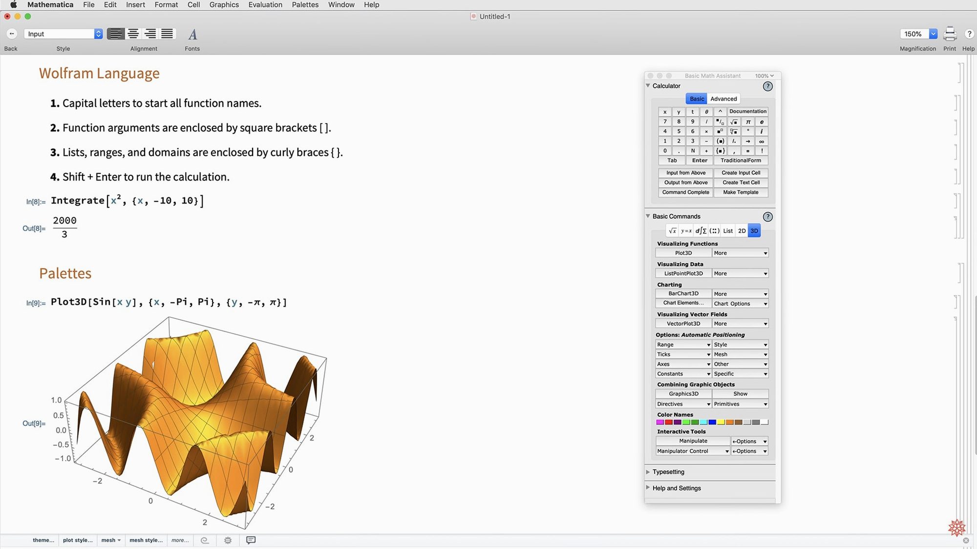
Mathematica is a technical computing environment that handles symbolic algebra, arbitrary-precision numerics, and data visualisation inside a single Wolfram Language workflow.
Who uses it, and for what?
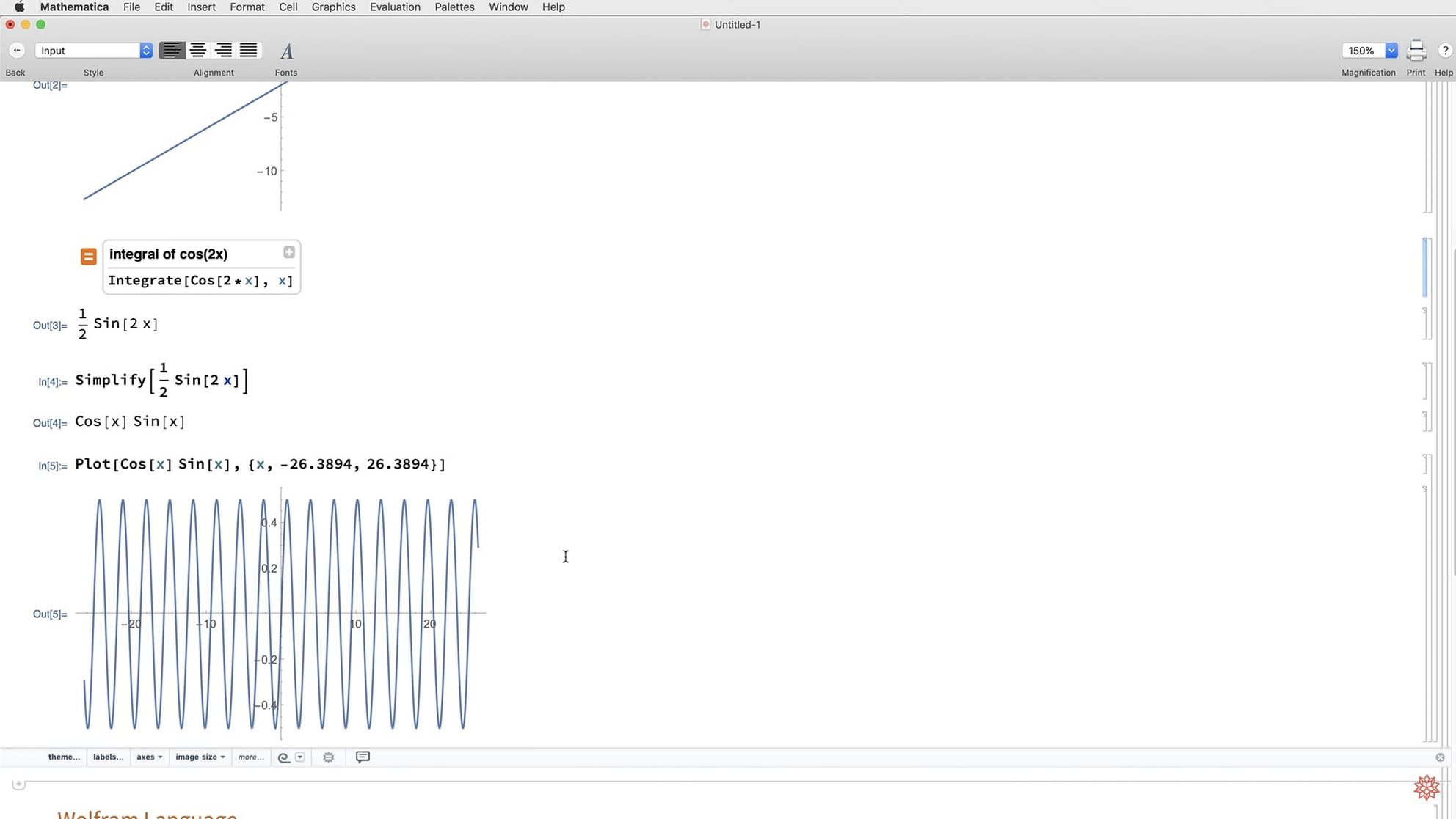
Engineers, mathematicians, and quantitative researchers use it to manipulate equations symbolically, run high-precision numerical simulations, and build interactive reports. Students encounter it in calculus, linear algebra, and physics courses where seeing the steps matters as much as the final result.
Does it only do maths?
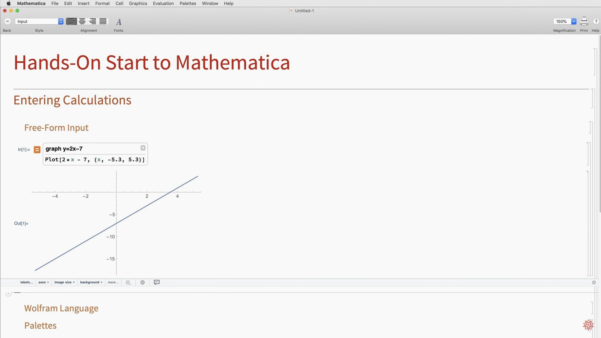
No. The system pulls in external data, processes text and images, and constructs graphical interfaces — all through the same notebook format. Natural-language input lets you type a question in plain English and get a computed answer without knowing the exact function name.
Where does it run?
The desktop app requires macOS 12 or later, with native support for both Intel and Apple Silicon Macs. Work also syncs to Wolfram Cloud and the iOS companion app, so a notebook started on a Mac can be reviewed or edited on a mobile device.
How Mathematica fits with macOS and other tools
Mathematica reads and writes dozens of formats, which makes it less of an island than it first appears. Drag a CSV or Excel file onto the dock icon and it lands in a notebook as a dataset ready for ListPlot or LinearModelFit. Image files import directly — PNG, JPEG, TIFF, and FITS for astronomy work — and the image processing functions operate on them without an external editor. Audio imports as raw sample data you can Fourier-transform or filter with a single command.
On the export side, notebooks save to PDF through the standard macOS print sheet, preserving vector graphics at full resolution. The version 14.3 addition of Markdown export is quietly useful: a completed analysis can become a plain-text document that Git can diff, or a draft that slides into a static-site generator without retyping equations.
Wolfram Language ties into Python and R through external evaluation, and the 14.3 release sped up data transfer between them. You can train a scikit-learn classifier from inside a Mathematica notebook, pass the result back, and plot it with Wolfram's graphics system — all without leaving the single document. For Apple-specific workflows, RunThrough and ExternalEvaluate can shell out to command-line tools, though direct AppleScript or Shortcuts integration requires custom glue.
Copy and paste works two ways with LaTeX. Highlight a typeset expression in a notebook, copy it, and the clipboard holds valid LaTeX. Paste LaTeX from a paper and Mathematica interprets it as an expression you can evaluate immediately. This alone saves researchers from re-entering equations found in PDFs or Overleaf documents.
Dark mode now respects syntax and palette contrast
Dark mode, added in 14.3, is a genuine quality-of-life improvement for anyone working late. Syntax highlighting respects the system appearance setting, and the new standard colour palette adjusts automatically — a red line visible against a white background stays distinguishable on a dark one without manual tweaking.
The Hilbert transform and Lommel functions fill gaps in signal processing and optics respectively. Engineers analysing single-sideband modulation can call HilbertTransform directly instead of building it from Fourier primitives. Lommel functions simplify diffraction calculations that previously needed workarounds with hypergeometric series.
On the visualisation front, ListFitPlot removes the boilerplate of fitting a curve and then plotting it separately. Supply data points and a model, and the function returns a graphic with both the points and the fitted line or surface rendered in one step. The new surface plotting functions handle large meshes more gracefully, and the vector-based map output produces clean graphics at any zoom level — useful when a plot moves from screen to a printed poster.
LLMGraph is a small but telling addition: it constructs a graph from a text description using an LLM service, turning a phrase like "show the supply chain from lithium mining to battery production" into nodes and edges you can then analyse with the rest of the graph toolkit. The faster Python and R integration means iterative workflows — tweak a model, test it, plot it, repeat — feel less sluggish.
Workflow: cleaning and plotting experimental data
Start with a CSV file from a lab instrument — timestamps in column one, sensor readings in columns two through five. Drag the file into a notebook or use Import["path/to/data.csv"]. The result is a list of lists. Assign it to a variable: raw = Import["~/Desktop/sensor_log.csv"].
Inspect the first few rows with raw[[1;;5]]. Spot the header row and strip it: data = raw[[2;;-1]]. Convert string entries to numbers with data = ToExpression[data]. If the timestamp column uses an awkward format, DateObject with a format string parses it.
Plot all four sensor channels quickly to check for outliers: ListLinePlot[data[[All, {1, #}]] & /@ Range[2,5]]. One channel shows a spike that is clearly instrument noise. Filter it with a median window: MedianFilter[data[[All,3]], 5]. Replace the column with the cleaned values.
Now fit a model to channel three against time. The relationship looks logarithmic. Use NonlinearModelFit[data[[All, {1,3}]], a + b Log[x], {a, b}, x]. The output gives parameter estimates, standard errors, and goodness-of-fit statistics. Plot data and fit together with ListFitPlot — the version 14.3 function that shows points, the fitted curve, and a confidence band in a single graphic. Export the finished plot as a PDF for a report, and export the cleaned dataset as CSV to pass to a colleague who uses Excel.
A physicist's afternoon
A condensed-matter researcher has just pulled impedance spectroscopy data from a new sample. She opens Mathematica on her M3 MacBook Pro, imports the raw text files, and removes the calibration offset with a one-line subtraction across the complex-valued dataset. She writes a quick Manipulate to sweep through an equivalent-circuit model, adjusting resistor and capacitor values with sliders while the Nyquist plot updates in real time. The interactive widget reveals a second time constant she had not anticipated.
She grabs a screenshot of the Manipulate output using Shift-Cmd-4, but the real work happens when she copies the circuit parameters and pastes them into a LaTeX draft in a separate editor. Before leaving, she exports the notebook as Markdown and commits it alongside the raw data files. A collaborator in another lab can read the analysis steps without having Mathematica installed — the Markdown preserves the text, while the exported PNG plots and CSV files carry the numbers.
- Interface — full dark mode support and new standard colours tuned for light and dark environments
- Functions — Hilbert transforms, Lommel functions, and additional matrix decompositions
- Visualisation — ListFitPlot, enhanced surface plotting routines, vector-based maps, and mesh processing tools
- Integration — faster Python and R interop, ColumnwiseCombine, geodesic computation, LLMGraph, system model validation, and Markdown export
- macOS 12 or later
- Apple Silicon or Intel processor
Questions on file
What sorts of computation does Mathematica cover?
It covers symbolic manipulation of algebraic expressions, arbitrary-precision numerical computation, and 2D or 3D visualisation — all accessible through the Wolfram Language's thousands of built-in functions.
Which interface languages does the Mac version include?
The interface ships in English, Japanese, Simplified Chinese, Traditional Chinese, French, German, Italian, Spanish, Korean, Portuguese, Russian, Polish, Ukrainian, Lithuanian, Greek, and Vietnamese.
Sign in · Create an account to add a field note.
No field notes yet. A measurement, a version, a machine — they appear after moderation.